Trevisan’s construction

We have seen that quantum-proof strong randomness extractors are the correct functions to perform privacy amplification. Furthermore, we have shown that these functions are not just the desired mathematical objects, but can actually be constructed from a well-known class of functions: the class of two-universal functions. Finally, we presented two such families: Toeplitz hashing and the modified Toeplitz hashing.

In this section we will present an alternative method to obtain quantum-proof strong randomness extractors. Instead of constructing them from two-universal functions, we will use Luca Trevisan’s idea [9], which was later proved [10] to also work against quantum side information. Trevisan’s construction requires two things:

1. a weak design, and

2. a one-bit (quantum-proof strong) randomness extractor.

Remember that a randomness extractor always has two inputs: a weak source of randomness (an \(n\)-bit string) and a uniform seed (a \(d\)-bit string). Trevisan’s idea is the following: to obtain an \(m\)-bit \(\epsilon\)-close uniform string, we will call the one-bit extractor \(m\) times and concatenate all these bits. Each time, this extractor will receive some different bits from the uniform seed. What particular bits are used each time is determined by the weak design, which will guarantee that we use the whole input seed and the overlap between different calls is bounded.

The following figure graphically shows this construction.

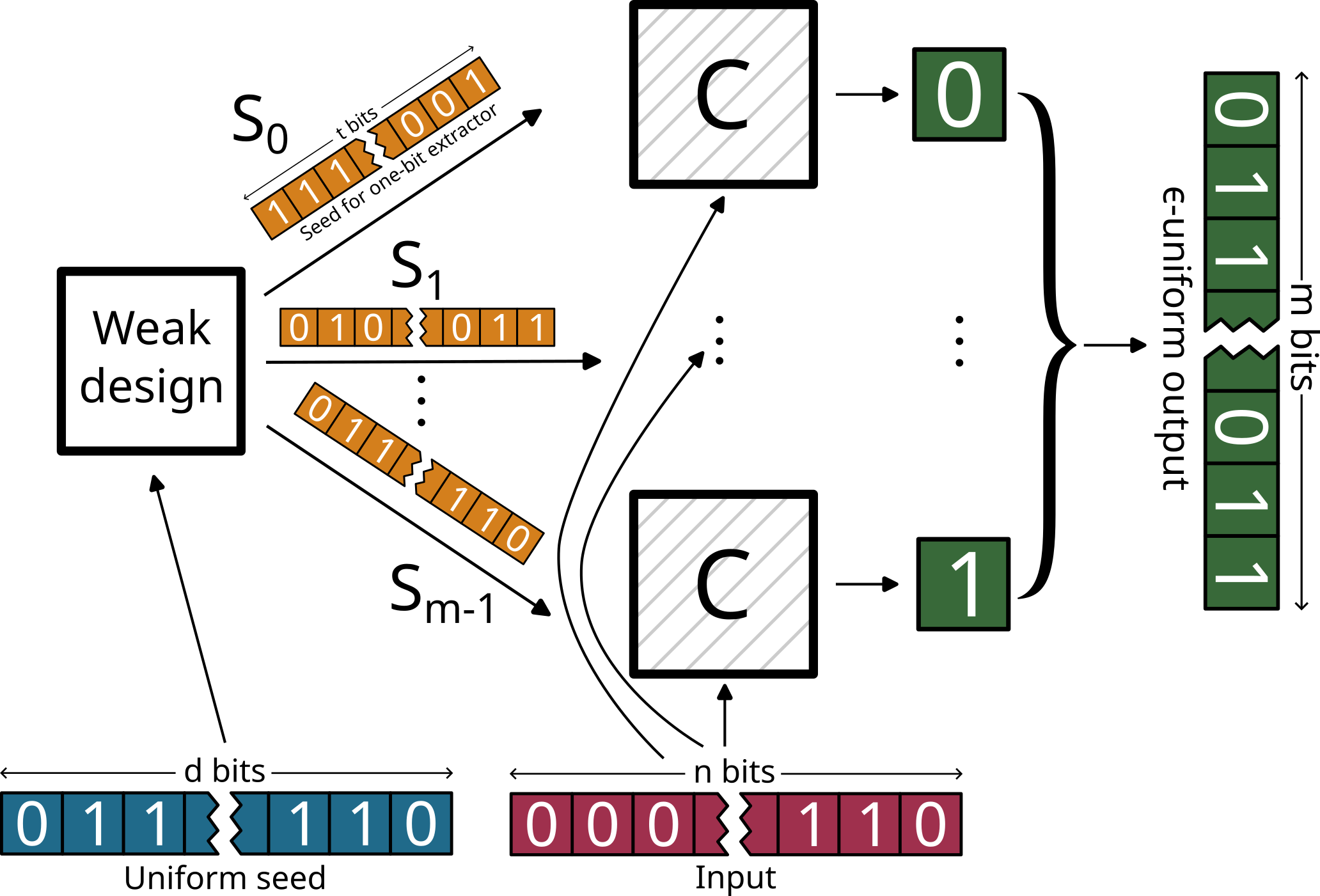
Trevisan’s construction diagram

Mathematically, if \(C:\{0,1\}^n\times\{0,1\}^t\rightarrow\{0,1\}\) is a quantum strong one-bit extractor, and the output of the weak design is a collection of indices \(S_0,\dots,S_{m-1}\), Trevisan’s construction is defined as

\[\text{Ext}(x,y):=C(x,y_{S_0})\dots C(x,y_{S_{m-1}})\,.\]

Complexity & seed length

It is not possible to talk about a generic complexity of the Trevisan’s construction since this will depend on the particular choice of the weak design and one-bit extractor. In practice, Trevisan’s construction is much slower that Toeplitz hashing. However, its main advantage is that, in some cases, it only requires a seed that grows logarithmically with the input length.

Let’s now dig into the details of these two required pieces to construct a Trevisan’s extractor. First we will have a look at combinatorial designs, and in particular weak designs, and then at two particular constructions of one-bit randomness extractors.

Combinatorial designs

Combinatorial designs ^{1 1}In the combinatorics literature, combinatorial designs are also called packings. are families of sets that are “almost disjoint”. They play an important role in pseudo random number generators (PRNG) and randomness extractors. Combinatorial designs are characterized by an upper bound on a metric that quantifies their overlap, and in the context of randomness extractors this is directly related to the length of the required uniform seed and the efficiency of the extractor: The larger this overlap, the smaller seed the construction requires, and the larger the entropy loss induced by the construction is. We will quantify this later.

Notation

Throughout this documentation, we use the following convention: \(\left[d\right]\) denotes a set of size \(\left|\left[d\right]\right|=d\) with set elements \(\{0,\dots,d-1\}\), and \(\log\) is always base 2 (unless explicitly stated otherwise).

A family of sets \(C:=\big[S_0, S_1, \dots, S_{m-1}\big]\subset[d]\) is a standard \((m,t,r,d)\)-design if

1. For all \(i\), \(|S_i|=t\)

2. For all \(i\neq j\), \(|S_i\cap S_j|\leq \log r\)

Although this definition is widely used in the literature, it was proved by Raz et al. [11] that a weaker definition, hence the use of weak in the name, is still useful in the context of randomness extractors.

Weak designs

A family of sets \(W:=\big[S_0, S_1, \dots, S_{m-1}\big]\subset[d]\) is a weak \((m,t,r,d)\)-design if

1. For all \(i\), \(|S_i|=t\)

2. For all \(i\), \(\sum_{j=0}^{i-1}2^{|S_i\cap S_j|}\leq rm\)

Note that this definition implies that every standard design is also a weak design, but not conversely.

Proof

\[\sum_{j=0}^{i-1}2^{|S_i\cap S_j|}\leq\sum_{j=0}^{i-1}2^{\log r}=\sum_{j=0}^{i-1}r\leq \sum_{j=0}^{m-1} r=rm\,,\]

where in the first inequality we used the definition of standard design

A basic construction

With the definition above, if we are given a family of sets, we can easily verify if it is indeed a weak design or not. In this section, however, we want to address a different problem: given a number of required sets of a fixed size with set elements from a particular set, how can we construct such a weak design? This is exactly the kind of problem we will face when trying to construct a Trevisan’s extractor.

A basic construction is possible making use of polynomials over a finite field \(\text{GF}(t)\). Every set \(S_p\) is indexed by a polynomial \(p\,:\,\text{GF}(t)\rightarrow\text{GF}(t)\). A weak \((m,t,r,d)\)-design has \(m\) sets of size \(t\) with set elements from \([d]\). Hence, we need \(m\) such polynomials.

The \(j\)-th polynomial is given by

\[p_j(\gamma)=\sum_{i=0}^c\alpha_j(i)\gamma^i\,,\quad \text{with}\quad \alpha_j(i)=\left\lfloor\frac{j}{t^i}\right\rfloor\!\! \mod t\,,\quad\text{and}\quad c=\left\lceil\frac{\log m}{\log t}-1\right\rceil\,,\]

for \(j\in[m]\).

Example \((m=6,\: t=2)\)

\begin{gather} c = \left\lceil\frac{\log 6}{\log 2}-1\right\rceil=2\\ p_j(\gamma) = \sum_{i=0}^2\alpha_j(i) \gamma^i=\alpha_{j}(0)+\alpha_j(1)\gamma+\alpha_j(2)\gamma^2\\ p_0=0,\quad p_1=1,\quad p_2=\gamma,\quad p_3=1+\gamma,\quad p_4=\gamma^2,\quad p_5=1+\gamma^2 \end{gather}

Once we have computed all the \(m\) polynomials, the elements of the set \(S_j\) are all the pairs of values

\[S_j=S_{p_j}:=\Big\{\big(z, p_j(z)\big)\;:\; z\in\text{GF}(t)\Big\}\,,\]

where \(p_j(z)\in\text{GF}(t)\) is the evaluation of the \(j\)-th polynomial at value \(z\).

Example \((m=6,\: t=2)\)

\[\begin{split}S_0=\Big\{\big(0, p_0(0)\big),\;\big(1, p_0(1)\big)\Big\}=\Big\{\big(0, 0\big),\;\big(1, 0\big)\Big\}\\ S_1=\Big\{\big(0, p_1(0)\big),\;\big(1, p_1(1)\big)\Big\}=\Big\{\big(0, 1\big),\;\big(1, 1\big)\Big\}\\ S_2=\Big\{\big(0, p_2(0)\big),\;\big(1, p_2(1)\big)\Big\}=\Big\{\big(0, 0\big),\;\big(1, 1\big)\Big\}\\ S_3=\Big\{\big(0, p_3(0)\big),\;\big(1, p_3(1)\big)\Big\}=\Big\{\big(0, 1\big),\;\big(1, 0\big)\Big\}\\ S_4=\Big\{\big(0, p_4(0)\big),\;\big(1, p_4(1)\big)\Big\}=\Big\{\big(0, 0\big),\;\big(1, 1\big)\Big\}\\ S_5=\Big\{\big(0, p_5(0)\big),\;\big(1, p_5(1)\big)\Big\}=\Big\{\big(0, 1\big),\;\big(1, 0\big)\Big\}\end{split}\]

There is one last step. Remember that we want our sets to have elements from \([d]\), but right now we have pairs of elements from \(\text{GF}(t)\). We can easily map, assuming that \(d=t^2\), \([t]\times [t]\rightarrow [d]\), for example, with \((i,j)\mapsto i + j\cdot t\).

Example \((m=6,\: t=2)\)

\[\begin{split}S_0=\Big\{\big(0, 0\big),\;\big(1, 0\big)\Big\}=\{0, 1\}\\ S_1=\Big\{\big(0, 1\big),\;\big(1, 1\big)\Big\}=\{2, 3\}\\ S_2=\Big\{\big(0, 0\big),\;\big(1, 1\big)\Big\}=\{0, 3\}\\ S_3=\Big\{\big(0, 1\big),\;\big(1, 0\big)\Big\}=\{2, 1\}\\ S_4=\Big\{\big(0, 0\big),\;\big(1, 1\big)\Big\}=\{0, 3\}\\ S_5=\Big\{\big(0, 1\big),\;\big(1, 0\big)\Big\}=\{2, 1\}\\\end{split}\]

The weak design \(W\) is the collection of all these sets \(S_j\)

Example \((m=6,\: t=2)\)

\[W = \big[\{0,1\}, \{2, 3\}, \{0, 3\}, \{2, 1\}, \{0, 3\}, \{2, 1\}\big]\]

Block design

A Trevisan’s extractor that takes \(n\) bits and outputs \(m\) bits constructed from a weak \((m,t,r,d)\)-design and a quantum-proof \((k,\epsilon)\)-strong extractor is a quantum-proof \((k+rm, m\epsilon)\)-strong extractor. Now it is clearer that the overlap parameter \(r\) determines the entropy loss of the construction induced by the weak design. Ideally, if we have \(k\) bits of entropy we would also like to extract \(k\) bits, so we can quantify the entropy loss as \(k-m\). In the case of the Trevisan’s construction we have an overhead term due to the weak design so the entropy loss is actually \(k+rm-m=k+m(r-1)\). Only when \(r=1\) the entropy loss of the Trevisan’s construction is roughly the same as the entropy loss of the underlying one-bit extractor. The basic construction described above has an overlap parameter of \(r=2e\). This means that the entropy loss induced by the weak design grows linearly with the output length as \(m(2e-1)\approx4.4m\).

Is it possible to construct a weak design with \(r=1\) that minimizes the entropy loss? The answer is yes, and we can construct it by combining multiple basic weak designs with an arbitrary parameter \(r\). This is called a block design. Let’s use the following representation to better visualize this construction: A basic weak design \(W_B = [S_0, S_1, \dots, S_{m-1}]\) can be depicted by a binary matrix of dimensions \(m\times d\), where \(w_{ij}=1\) if \(j\in S_i\).

Example weak design \((m=6,\: t=2)\) matrix

The weak design from the previous example can also be written as the following \(6\times4\) matrix.

\[\begin{split}W_B = \begin{pmatrix} 1 & 1 & 0 & 0 \\ 0 & 0 & 1 & 1 \\ 1 & 0 & 0 & 1 \\ 0 & 1 & 1 & 0 \\ 1 & 0 & 0 & 1 \\ 0 & 1 & 1 & 0 \end{pmatrix}\end{split}\]

Then, the binary matrix of the block design \(W\) is constructed placing \(l+1\) matrices of basic weak designs in the diagonal, i.e.,

\[\begin{split}W = \begin{pmatrix} W_{B,0} & & \\ & \ddots & \\ & & W_{B,l} \end{pmatrix}\,.\end{split}\]

The first thing we need to determine is how many such basic weak designs we need. The number \(l\) depends on the number of sets \(m\), the size of the sets \(t\), and the overlap parameter \(r\) of the underlying construction

\[l = \max \left\{1, \left\lceil \frac{\log(m-r) - \log(t-r)}{\log r - \log(r-1)} \right\rceil \right\}\,.\]

Not surprisingly, for larger overlap parameters \(r\) we need to combine more weak designs to obtain the desired \(r=1\).

Minimum size of sets

Note that this construction is only well defined for \(m \geq t >r\). In particular, if we use the basic weak design construction explained above with \(r=2e\) to construct a block design the smallest number of sets is 6 and the smallest size of sets is 7 (since this number needs to be a prime number).

Then, we need to determine the number of sets \(m_i\) for each instance of the basic weak design

\[\begin{split}\begin{align} m_i &= \left\lceil \sum_{j=0}^i n_j \right\rceil - \sum_{j=0}^{i-1}m_j \quad \text{for}\; 0 \leq i \leq l-1\,, \\ m_l &= m - \sum_{j=0}^{l-1} m_j\,, \end{align}\end{split}\]

where the auxiliary numbers \(n_i\) are given by

\[n_i = \left( 1 - \frac{1}{r}\right)^i \left(\frac{m}{r} - 1 \right)\,.\]

Example block design \((m=6,\: t=7)\)

First we determine \(l\):

\[l = \max \left\{ 1, \left\lceil \frac{\log(6-2e)-\log(7-2e)}{\log(2e) - \log(2e-1)} \right\rceil \right\} = \max \{1, -5\} = 1\]

Then we compute \(m_0\) and \(m_1\):

\[\begin{split}\begin{align} n_0 &= \frac{6}{2e} - 1 \approx 0.10 \\ m_0 &= \lceil n_0 \rceil = 1 \\ m_1 &= 6 - 1 = 5 \end{align}\end{split}\]

We need to obtain the two weak designs \(W_0\) and \(W_1\) using the basic construction:

\[W_0 = [\{0,1,2,3,4,5,6\}]\]

\[\begin{split}\begin{align} W_1 = [&\{0,1,2,3,4,5,6\}, \{7,8,9,10,11,12,13\}, \{14,15,16,17,18,19,20\}, \\ &\{21,22,23,24,25,26,27\}, \{28,29,30,31,32,33,34\}] \end{align}\end{split}\]

We are not done yet. The block design construction was defined in terms of the binary matrix representation. Placing the basic weak designs in the diagonal of the matrix is equivalent to shifting the \(i\)-th weak design indices by \(it^2\). In this case the final block design is:

\[\begin{split}\begin{align} W = [&\{0,1,2,3,4,5,6\}, \{49,50,51,52,53,54,55\}, \{56,57,58,59,60,61,62\}, \\ &\{63,64,65,66,67,68,69\}, \{70,71,72,73,74,75,76\}, \{77,78,79,80,81,82,83\}] \end{align}\end{split}\]

One-bit extractors

There is not a lot to tell about quantum-proof strong one-bit randomness extractors. Everything we said in the seeded extractors section also applies here. The only difference is that the output, instead of an \(m\)-bit string, is a single bit. Mathematically,

\[\text{Ext}_1:\{0,1\}^n\times\{0,1\}^t\rightarrow\{0,1\}\,.\]

It takes a weak random source \(X\), a bit string of length \(n\), and a uniform seed \(Y\), a bit string of length \(t\), and outputs a single bit.

We will explain the current one-bit extractors included in randextract.

Notation

We denote the length of the seed required by the one-bit extractor with \(t\) instead of \(d\) to distinguish from the seed length used by the Trevisan’s construction. We will always have that \(t<d\).

XOR one-bit extractor

The XOR one-bit extractor is defined as the function

\begin{align} \text{Ext}_1: \{0,1\}^n\times [n]^l&\rightarrow \{0,1\}\\ (x, y) &\mapsto \bigoplus_{i=0}^{l-1} x_{y_i}\,. \end{align}

In order to write down the function more compactly, the seed \(y\) here is formed by \(l\) integers from \([n]\) instead of an \(l\)-bit string. In words, this extractor takes the whole input \(x\), selects only \(l\) bits from it using the seed \(y\), and computes the parity ^{2 2}Parity of a bit string refers to whether it contains an odd or even number of 1-bits. The bit string has “odd parity” (1), if it contains odd number of 1-bits and has “even parity” (0) if it contains even number of 1-bits. of those selected bits.

Example \((n=20,\: l=7)\)

\begin{align} x &= [0, 1, 1, 1, 0, 0, 1, 1, 0, 1, 1, 0, 1, 0, 0, 1, 0, 0, 0, 0]\\ y &= [0, 10, 13, 15, 17, 14, 5]\\ \text{Ext}_1(x,y) &= x_0\oplus x_{10}\oplus x_{13}\oplus x_{15}\oplus x_{17}\oplus x_{14}\oplus x_5 = 0 \end{align}

Polynomial hashing one-bit extractor

What we denote here as polynomial hashing is actually a concatenation of two hash functions. The seed used by the one-bit extractor, \(y\in\{0,1\}^{2t}\), is split into two, i.e., \(y=(\alpha|\beta)\), where both \(\alpha,\beta\in\{0,1\}^t\). The extractor is the following function

\[\text{Ext}_1(x,y) := \bigoplus_{i=0}^{t-1} \beta_i p_\alpha(x)_i\,.\]

In words, the output is the parity of the bitwise product between \(p_\alpha(x)\), the first hash function, and the second half of the seed \(\beta\). Note that the first hash function only uses the first half of the seed, \(\alpha\), but it takes the whole input \(x\).

The name of polynomial hashing comes precisely from this first hashing. In particular, to compute \(p_\alpha(x)\), first we split the \(n\)-bit input string \(x\) in \(l\) blocks of length \(t\), i.e.,

\[x = (x_0,x_1,\dots,x_{l-1})\,.\]

Padding with 0s

Note that because \(n\) might not be divisible by \(l\), the last block \(x_{l-1}\) may be of a size smaller than \(t\). This is avoided by padding the block with 0s to get the right size.

Then, each block \(x_i\) is interpreted as an element of a finite field \(\text{GF}(2^t)\), and the hash function reduces to a polynomial evaluation

\[p_\alpha(x) := \sum_{i=0}^{l-1}x_i\alpha^{l-i-1}\,.\]

Polynomials to bit strings

Note that there is not a unique way of converting an element of an extended finite field to a bit string. In particular, we are free to choose the irreducible polynomial \(\text{P}\) used for all the arithmetic operations with elements of the field. In our library, unless manually specified, and in the next example we use the irreducible polynomials with the minimum possible number of non-zero terms. Once the irreducible polynomial is fixed, we use the notation \(\text{GF}(2^q)/\big<P\big>\), and this fixes a mapping from a polynomial representation to an integer representation, which we can use to obtain a corresponding bit string.

Example polynomial hashing \((n=25,\: t=12,\: l=3)\)

Notation

To avoid confusion since we are denoting the input as \(x\), the indeterminate or variable of the polynomial is here denoted by the greek letter \(\gamma\).

Let’s first write down the input and the seed, and express the first half of the seed \(\alpha\) as a polynomial of the finite field \(\text{GF}(2^{12})\). For the arithmetic calculations we are using the following irreducible polynomial: \(\gamma^{12} + \gamma^3 + 1\). We will use the notation \(\text{GF}(2^{12})/\big<\gamma^{12} + \gamma^3 + 1\big>\) to explicitly emphasize the irreducible polynomial.

\begin{align} x &= \begin{bmatrix} 1 & 0 & 1 & 0 & 1 & 1 & 1 & 1 & 1 & 0 & 1 & 0 & 0 & 1 & 1 & 1 & 0 & 0 & 1 & 1 & 0 & 0 & 0 & 0 & 0 \end{bmatrix} \\ y &= \begin{bmatrix} 0 & 0 & 1 & 0 & 0 & 1 & 1 & 1 & 0 & 0 & 1 & 1 & 1 & 0 & 0 & 1 & 0 & 0 & 1 & 0 & 1 & 1 & 1 & 1 \end{bmatrix} \\ \alpha &= \begin{bmatrix} 0 & 0 & 1 & 0 & 0 & 1 & 1 & 1 & 0 & 0 & 1 & 1 \end{bmatrix} = \gamma^9+\gamma^6+\gamma^5+\gamma^4+\gamma+1 \in \text{GF}(2^{12})\\ \beta &= \begin{bmatrix} 1 & 0 & 0 & 1 & 0 & 0 & 1 & 0 & 1 & 1 & 1 & 1 \end{bmatrix} \\ \end{align}

Now we split the input into 3 blocks of size 12 and we pad the last block with additional 0s

\begin{align} x = \Big[&\begin{bmatrix}1 & 0 & 1 & 0 & 1 & 1 & 1 & 1 & 1 & 0 & 1 & 0 \end{bmatrix},\\ &\begin{bmatrix}0 & 1 & 1 & 1 & 0 & 0 & 1 & 1 & 0 & 0 & 0 & 0 \end{bmatrix},\\ &\begin{bmatrix}0 & 0 & 0 & 0 & 0 & 0 & 0 & 0 & 0 & 0 & 0 & 0 \end{bmatrix}\Big]\,. \end{align}

We write each block as an element of \(\text{GF}(2^{12})\)

\begin{align} x = \big[& \gamma^{11} + \gamma^9 + \gamma^7 + \gamma^6 + \gamma^5 + \gamma^4 + \gamma^3 + \gamma,\\ & \gamma^{10} + \gamma^9 + \gamma^8 + \gamma^5 + \gamma^4,\\ & 0\big]\,. \end{align}

We need to compute a few terms before being able to use the formula for the first hash function. In particular, we need to compute \(\alpha^2\), \(x_0\alpha^2\) and \(x_1\alpha\) \(\in\text{GF}(2^{12})/\big<\gamma^{12} + \gamma^3 + 1\big>\)

\begin{align} \alpha^2 &= (\gamma^9+\gamma^6+\gamma^5+\gamma^4+\gamma+1)(\gamma^9+\gamma^6+\gamma^5+\gamma^4+\gamma+1) \\ &= \gamma^{18}+\gamma^{12}+\gamma^{10}+\gamma^8+\gamma^2+1 \\ &= (\gamma^6+1)(\gamma^{12}+\gamma^3+1) + (\gamma^{10}+\gamma^9+\gamma^8+\gamma^6+\gamma^3+\gamma^2) \\ &= \gamma^{10}+\gamma^9+\gamma^8+\gamma^6+\gamma^3+\gamma^2 \end{align}

In the last step we reduce the expression dividing it by the irreducible polynomial. Similary, we compute the other two terms.

\begin{align} x_0\alpha^2 &= (\gamma^{11}+\gamma^9+\gamma^7+\gamma^6+\gamma^5+\gamma^4+\gamma^3+\gamma)(\gamma^{10}+\gamma^9 +\gamma^8+\gamma^6+\gamma^3+\gamma^2) \\ &= \gamma^{21}+\gamma^{20}+\gamma^{18}+\gamma^{17}+\gamma^{13}+\gamma^{10}+\gamma^7+\gamma^5+\gamma^4+ \gamma^3 \\ &= (\gamma^9+\gamma^8+\gamma^6+\gamma^5+\gamma+1)(\gamma^{12}+\gamma^3+1) + (\gamma^{11}+\gamma^{10}+\gamma^7 +\gamma^6+\gamma+1)\\ &= \gamma^{11}+\gamma^{10}+\gamma^7+\gamma^6+\gamma+1 \end{align}

\begin{align} x_1\alpha &= (\gamma^{10}+\gamma^9+\gamma^8+\gamma^5+\gamma^4)(\gamma^9+\gamma^6+\gamma^5+\gamma^4+\gamma+1) \\ &= \gamma^{19}+\gamma^{18}+\gamma^{17}+\gamma^{16}+\gamma^{13}+\gamma^{12}+\gamma^6+\gamma^4 \\ &= (\gamma^7+\gamma^6+\gamma^5+\gamma^4+\gamma+1)(\gamma^{12}+\gamma^3+1) + (\gamma^{10}+\gamma^9+\gamma^8 +\gamma^5+\gamma^4+\gamma^3+\gamma+1) \\ &= \gamma^{10}+\gamma^9+\gamma^8+\gamma^5+\gamma^4+\gamma^3+\gamma+1 \end{align}

Finally, we compute the hash using the above formula

\begin{align} p_\alpha(x)&=\sum_{i=0}^{2}x_i\alpha^{2-i}=x_0\alpha^2+x_1\alpha+x_2\\ &= \gamma^{11}+\gamma^{10}+\gamma^7+\gamma^6+\gamma+1+\gamma^{10}+\gamma^9+\gamma^8+\gamma^5+\gamma^4+\gamma^3 +\gamma+1 \\ &= \gamma^{11}+\gamma^9+\gamma^8+\gamma^7+\gamma^6+\gamma^5+\gamma^4+\gamma^3 \\ &= \begin{bmatrix} 1 & 0 & 1 & 1 & 1 & 1 & 1 & 1 & 1 & 0 & 0 & 0 \end{bmatrix}\,. \end{align}

The last step is compute the parity of the bitwise product of previous output with the second half of the seed

\begin{align} \text{Ext}_1(x,y) &= \bigoplus_{i=0}^{11} \beta_i p_\alpha(x)_i\\ &= \bigoplus [1, 0, 0, 1, 0, 0, 1, 0, 1, 1, 1, 1] \odot [1, 0, 1, 1, 1, 1, 1, 1, 1, 0, 0, 0]\\ &= \bigoplus [1, 0, 0, 1, 0, 0, 1, 0, 1, 0, 0, 0] = 0 \end{align}

For smaller examples you can also check the unit tests of this implementation.